---
title: "Tree phenology observations in Wauseon, Ohio"
date: 2024-06-12
author:
- name: Daniel Burcham
orcid: 0000-0002-1793-3945
description: "Using Shiny for R, explore dynamic visualizations of tree phenology recorded by Thomas Mikesell in Wauseon, Ohio between 1883 and 1912"
image: thomas_mikesell.jpg
format:
html
categories:
- bslib
- ggplot
- r
- shiny
- tidyverse
filters:
- shinylive
---
```{r}
#| code-fold: true
library(knitr)
knitr::opts_chunk$set(fig.width = 7, fig.align = "center",
fig.retina = 1, out.width = "90%",
collapse = TRUE)
```
## Hometown specials
I often think that I know everything about my origins in rural Ohio. As a child, I constantly roamed the roads and trails of my quiet
hometown on my bike, and I observed the rhythms of small town life
marked by planting, harvest, small talk, and public school calendars.
Outside of town, the land was shaped by generations of agriculture, and
everyone experienced some form of hardship as the world around us
changed. It was a quiet corner of the country where
nothing remarkable happened.
Given my familiarity with the territory, I am rarely surprised by
stories from my birthplace, but I recently discovered a person who lived
a quiet life in the area with a remarkable legacy - Thomas Mikesell.
Over several decades, he kept meticulous records about seasonal events
in the natural world. A keen student of phenology, he made thousands of
records of shoot expansion, flowering, fruiting, and leaf senescence for
hundreds of commodity crops, specialty crops, trees, and ornamental
plants around the turn of the 20th Century with accompanying notes about
weather conditions. In 1914, a detailed
[report](smith-1915-phenological_dates_and_meteorological_data_recorded_by_thomas_mikesell_between.pdf)
of Thomas Mikesell's life and work was published in the *Monthly Weather
Review Supplement*, and it offers some remarkable details about one
man's passionate side project:
> The observer, Thomas Mikesell, was born on the farm 1 mile north of
> where Wauseon, Ohio, now stands in Fulton County but then Lucas
> County. His parents, William and Margaret (Boyes) Mikesell, came from
> western Pennsylvania in April, 1837, and settled in the forest.
>
> He attended country schools until 14 years of age and then went to the
> high school at Wauseon, 1 mile distant. At that time the Wauseon High
> School had but two rooms. In June, 1863, he enlisted in Company H,
> Eighty-sixth Ohio Volunteer Infantry and served with it until February
> 10, 1864. After leaving the Army Mr. Mikesell resumed his high-school
> course and in 1866 his school days ended; not so his study of nature.
>
> For several winters Mikesell taught elementary school in Ohio, Iowa,
> and northern Missouri; then he returned to Wauseon in the fall of
> 1869. From this time on he worked on the farm, retiring from active
> life in the spring of 1902. In November, 1873, he married Miss Martha
> Heniman, but no children have come to this union.
>
> In 1889 he was elected secretary of the Fulton County Fair and for 16
> consecutive years he continued to serve in that capacity. In 1902 he
> was appointed a corn and wheat region observer by the United States
> Weather Bureau and that same year, because of failing health, he was
> obliged to give up his farm and move to Wauseon, where he still
> resides.
>
> The observations published in this present supplement are but a
> portion of the records that this one man maintained during his busy
> life. They constitute one of the most complete and reliable local
> records of which we have knowledge, as to the development of plant
> life and the migrations of birds and animals. Quietly, carefully,
> conscientiously, this man has merely kept his eyes open to see and
> systematically recorded the movements of nature about him year after
> year. He has done what thousands of other men might have done, but
> which no other one has done. The writer believes that science owes a
> great debt to such a man, that all honor is due him, and that the name
> of Thomas Mikesell should be set high among the faithful students of
> nature in this country.
## Exploring tree phenology
Mikesell brought a level of commitment and dedication rarely matched to
his hobby, and the biographer echoes the natural reaction of ordinary
people to such an extraordinary accomplishment. I certainly appreciate
the character required for such an undertaking. In life, we more
often seek quick rewards from meager investments, and it's always a
pleasure to see someone creating enduring value without an expectation
for immediate recognition. Similar examples of impressive amateur study,
like [Billy Barr](https://vimeo.com/182392548) at the Rocky Mountain Biological Laboratory, are
rare. In recent decades, Mikesell's valuable records have been
discovered and used by many scientists studying changes in the pattern
of natural events over time. I encountered the story and data in an
[article](https://doi.org/10.2307/2404467) attempting to predict the
timing of budburst for temperate tree species, and one interesting [study](https://doi.org/10.1371/journal.pone.0282635) compared
Mikesell's notes to more recent observations of trees on the same land.
Notably, they discovered that delayed fall leaf drop was largely
responsible for a longer growing season in recent years.
::: {.callout-tip collapse="true"}
## More about phenophases
To aid observations, the [USA National Phenology
Network](https://www.usanpn.org) developed standardized definitions for
some of the major phenophases (listed below). Mikesell's protocol may not have been equally detailed, but he probably, like many people, intuitively recognized and enjoyed observing repeating patterns in nature, especially if they coincided with other seasonal milestones in life.
**Breaking leaf buds**: One or more breaking leaf buds are visible on
the plant. A leaf bud is considered "breaking" once a green leaf tip is
visible at the end of the bud but before the first leaf from the bud has
unfolded to expose the leaf stalk (petiole) or leaf base.
**Leaves**: One or more live, unfolded leaves are visible on the plant.
A leaf is considered "unfolded" once its entire length has emerged from
a breaking bud, stem node, or growing stem tip so that the leaf stalk
(petiole) or leaf base is visible at its point of attachment to the
stem. Do not include any fully dried or dead leaves.
**Open flowers**: One or more open, fresh flowers are visible on the
plant. Flowers are considered "open" when the reproductive parts (male
stamens or female pistils) are visible between or within unfolded or
open flower parts (petals, floral tubes, or sepals). Do not include
wilted or dried flowers.
**Ripe fruit**: One or more ripe fruits are visible on the plant.
**Colored leaves**: One or more leaves show some of their typical
late-season color, or yellow or brown due to drought or other stresses.
Do not include small spots of color due to minor leaf damage or dieback
on branches that have broken. Do not include any fully dried or dead
leaves that remain on the plant.
**Falling leaves**: One or more leaves with typical late-season color,
or yellow or brown due to other stresses, are falling or have recently
fallen from the plant. Do not include fully dried or dead leaves that
remain on the plant for many days before falling.
:::
After discovering the data, I wanted to develop a new resource for my
arboriculture course showing the sequence of major phenophases among
various tree species. In my class, I often emphasize the importance of
informed expectations about seasonal tree growth and development. The
northern catalpa (*Catalpa speciosa*), for example, produces new leaves
very late in the spring, and one could easily assume, without knowing
the tree, that the delay was a serious concern. In becoming familiar
with a tree, it's also helpful to know the time it typically flowers,
develops fall color, or, perhaps, fruits. In Colorado, we often receive
heavy snow in the late spring and fall, and it isn't always desirable for trees to hold leaves when the storms typically occur. The
Mikesell records contain information about many of the trees grown in
Colorado landscapes, and, although the historical observations from Ohio may
not accurately predict contemporary tree phenology in Colorado, the data
contains many useful insights for anyone interested in the subject.
## Interactive Quarto documents with Shinylive
After digitizing the records for 26 woody species, I explored
visualizations of the data using violin plots, ensuring the observations
were properly formatted. Assuming it would be easier to plot a
continuous variable, I originally coded the Mikesell observations using
Julian days starting January 1 each year, but I converted them to
standard dates for readability, since `ggplot` accepts dates on an axis.
Next, I overlayed a jittered plot of individual observations using small
circle markers with opacity corresponding to the year of observation. If
the phenophases were consistently happening earlier or later each year,
the opacity mapping should produce an obvious color gradient, but the
gray colors for individual markers were clearly unorganized and showed
stochastic variation in the timing of events each year. Last, I added a
large circle marker depicting the median date of the phenophase for each
species. After creating the basic plot elements, I edited the plot style
to improve its appearance, and I reordered the display of species on the
y-axis by sorting the median phenophase date from earliest to latest.
```{r fig-dev, echo=TRUE, warning=FALSE, error=FALSE}
#| code-fold: true
#| fig-height: 6.5
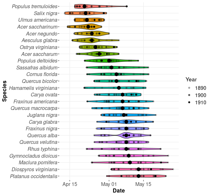
#| fig-cap: "Calendar dates Thomas Mikesell observed breaking leaf buds for various tree species in Wauseon, Ohio."
library(tidyverse)

data <- read.csv("Mikesell_Phenology_Data.csv", header = TRUE, na.strings = "999") |>
  mutate(bud_burst = as.Date(bud_burst,format="%j"),
         first_leaf = as.Date(first_leaf,format="%j"),
         full_leaf = as.Date(full_leaf,format="%j"),
         open_flowers = as.Date(open_flowers,format="%j"),
         ripe_fruit = as.Date(ripe_fruit,format="%j"),
         colored_leaves = as.Date(colored_leaves,format="%j"),
         leaves_dropped = as.Date(leaves_dropped,format="%j"))

ggplot(data, aes(bud_burst,reorder(species, bud_burst, FUN = median, na.rm = TRUE))) +
  geom_violin(aes(fill = reorder(species, bud_burst, FUN = median, na.rm = TRUE)), show.legend = FALSE, na.rm = TRUE) +
  stat_summary(fun = "median", size = 3.5, geom = "point", na.rm = TRUE) +
  geom_jitter(aes(alpha = year), height = 0, width = 0.2, na.rm = TRUE) +
  labs(
    x = "Date",
    y = "Species",
    alpha = "Year"
  ) +
  scale_y_discrete(limits=rev) +
  theme(axis.text.y = element_text(face="italic",size=12),
        axis.text.x = element_text(size=12),
        axis.title = element_text(face="bold",size=13),
        legend.text = element_text(size=12),
        legend.title = element_text(size=13),
        panel.background = element_rect(fill="white"),
        panel.grid.major = element_line(color="gray93"))
```
Although I liked the presentation of information in the figure, I would
need a lot of room for visual summaries of all seven phenophases
for 26 different species. Instead, I thought it would be better to
display everything dynamically in a single interactive plot based on a
user-selected phenophase. Although I had never developed such an
application in R, I wanted to use this as a reason to learn more about
Shiny apps. Shiny, developed in 2013, creates reactive web applications
in R, and, with some direction from other R users in my department, I used
Posit's Shiny
[tutorial](https://shiny.posit.co/r/getstarted/shiny-basics/lesson1/index.html)
to learn the basic principles. Essentially, there are three components
of a Shiny app:
- a user-interface (`ui`) object defines the app's layout and
appearance
- a server (`server`) function contains instructions for rendering app
components
- a call to the `shinyApp` function builds the app using `ui` and
`server` as inputs
```{r basic-shiny, echo=TRUE, eval=FALSE}
library(shiny)

ui <- ...

server <- ...

shinyApp(ui, server)
```
The Posit tutorial gives a detailed summary of the process for building
a local app with everything contained in a single `app.R` script. With
the file in its own directory, you can run the app by giving the
name of the directory to the `runApp` function or, in RStudio, you can
simply click on the Run App button at the top of the script editor
window.
### Creating a user interface
Although the Shiny package contains functions for controlling the
appearance of an app, often relying on the `fluidPage` and related
layout functions, most now recommend using the `bslib` package for its
superior style themes and interactive features. For my user interface, I
chose a standard sidebar layout with a collapsible sidebar on the left for user
input and a larger main area on the right for displaying the main app
content. In my code, the `page_sidebar` function requires three main
arguments, including a display name for the Shiny app (`title`),
control widgets for handling user input in the sidebar (`sidebar`), and
an unassigned R object for rendering the plot in the main area
(`plotOutput`). Notably, the first argument of the `plotOutput` function specifies the name of the object generated by the server function (`"phenophasePlot"`) for display in the app.
```{r ui-demo, echo=TRUE, eval=FALSE}
library(bslib)
library(shiny)

ui <- page_sidebar(
  title = "Mikesell Phenology Data",
  sidebar = radioButtons("radio","Select phenophase",
                         choices = c("Breaking leaf buds" = "bud_burst",
                                     "First leaf" = "first_leaf",
                                     "Full leaf" = "full_leaf",
                                     "Open flowers" = "open_flowers",
                                     "Ripe fruit" = "ripe_fruit",
                                     "Colored leaves" = "colored_leaves",
                                     "Leaves dropped" = "leaves_dropped"),
                         selected = "bud_burst"),
  plotOutput("phenophasePlot",width="100%")
)
```
For a control widget, I used radio buttons to let users select a
phenophase to display in the plot. In general, the widget functions
require two mandatory arguments, including a name (`"radio"`) and a display
label (`"Select phenophase"`), both specified as character strings, for
the user interface, and a number of additional inputs depending
on the type of widget. In my case, I
specified the list of possible choices for the radio buttons with the displayed names matched to
values (i.e., variable names) used in the code, and I set the first choice as the initially
selected value. The Shiny [function
reference](https://shiny.posit.co/r/reference/shiny/latest/) contains
extensive and detailed documentation related to Shiny UI layout and
inputs.
### Server structure and logic
The server function uses two list-like main arguments, `input` and `output`. The `input` object stores the current value of control widgets used by the app, accessed using the names assigned in the `ui` object. For example, I can access the user-selected phenophase using `input$radio`, and I used a switch function to match the input to a list of possible values. The switch function executes the code statements corresponding to the matching case, which, in my case, simply selects the variables needed to create the figure. I assigned the output to a new variable `dataInput`, and I made the entire statement a reactive expression to ensure the code section will be executed every time the control widget changes.
After creating the input data set, I assigned the output of the code previously developed for the figure to an element in the `output` object (`phenophasePlot`). The name of the element matches the one listed for display in the `ui` object. To create the type of reactive output expected, I wrapped the `ggplot` and related statements with the `renderPlot` function, and I had to define the plot variables implicitly in the corresponding lines of code to make everything work dynamically. For the input data, I called the reactive expression as a function, and I changed the statements corresponding to the phenophase observations to the current value stored in the control widget.
```{r server-demo, echo=TRUE, eval=FALSE}
library(shiny)
library(tidyverse)

server <- function(input, output) {

  dataInput <- reactive({
    switch(input$radio,
           bud_burst = phenoData[,c("year","species","bud_burst")],
           first_leaf = phenoData[,c("year","species","first_leaf")],
           full_leaf = phenoData[,c("year","species","full_leaf")],
           open_flowers = phenoData[,c("year","species","open_flowers")],
           ripe_fruit = phenoData[,c("year","species","ripe_fruit")],
           colored_leaves = phenoData[,c("year","species","colored_leaves")],
           leaves_dropped = phenoData[,c("year","species","leaves_dropped")])
  })

  output$phenophasePlot <- renderPlot({
    ggplot(dataInput(), aes(.data[[input$radio]],reorder(species, .data[[input$radio]], FUN = median, na.rm = TRUE))) +
      geom_violin(aes(fill = reorder(species, .data[[input$radio]], FUN = median, na.rm = TRUE)), show.legend = FALSE, na.rm = TRUE) +
      stat_summary(fun = "median", size = 3.5, geom = "point", na.rm = TRUE) +
      geom_jitter(aes(alpha = year), height = 0, width = 0.2, na.rm = TRUE) +
      labs(
        x = "Date",
        y = "Species",
        alpha = "Year"
      ) +
      scale_y_discrete(limits=rev) +
      theme(axis.text.y = element_text(face="italic",size=12),
            axis.text.x = element_text(size=12),
            axis.title = element_text(face="bold",size=13),
            legend.text = element_text(size=12),
            legend.title = element_text(size=13),
            panel.background = element_rect(fill="white"),
            panel.grid.major = element_line(color="gray93"))
  })
}
```
### Deploying the app
Now, the app worked well locally, but I wanted to find a reliable workflow for deploying the app to the web, since I want to share the app with people unfamiliar with R. As it turns out, the options for web deployment (e.g., [shinyapps.io](https://www.shinyapps.io), Shiny Server) all require hosting the app on a web server running R. Since server administration is a complex task, I prefer to avoid it, if possible. Fortunately, several brilliant developers have recently created tools allowing anyone to run R *in the browser*! By some unfathomable magic, the `shinylive` package, relying on [WebR](https://docs.r-wasm.org/webr/latest/), can be used to create serverless Shiny apps. That's right - no server needed! Since I use Quarto markdown, I had to install the Quarto Extension for `shinylive` by running `quarto add quarto-ext/shinylive` in the terminal. To insert a Shiny app in an interactive Quarto document, I added a filter key for `shinylive` in the document's YAML header, and I added a code block marked with `{shinylive-r}` and a `#| standalone: true` option. Below, you can explore the code and interactive Shiny app in adjacent windows. If you'd like, you can also edit the code and restart the app using the play button at the top. Try it out for yourself!
I hope you're proud, Thomas Mikesell.
```{shinylive-r}
#| standalone: true
#| viewerHeight: 750
#| components: [editor, viewer]
#| layout: vertical
# Load packages
library(bslib)
library(shiny)
library(tidyverse)
# Import and wrangle data
download.file("https://raw.githubusercontent.com/danielburcham/arbdatascience/master/Mikesell_Phenology_Data.csv", "Mikesell_Phenology_Data.csv")
phenoData <- read.csv("Mikesell_Phenology_Data.csv", header = TRUE, na.strings = "999") |>
mutate(bud_burst = as.Date(bud_burst,format="%j"),
first_leaf = as.Date(first_leaf,format="%j"),
full_leaf = as.Date(full_leaf,format="%j"),
open_flowers = as.Date(open_flowers,format="%j"),
ripe_fruit = as.Date(ripe_fruit,format="%j"),
colored_leaves = as.Date(colored_leaves,format="%j"),
leaves_dropped = as.Date(leaves_dropped,format="%j"))
# Define user interface
ui <- page_sidebar(
title = "Mikesell Phenology Data",
sidebar = radioButtons("radio","Select phenophase",
choices = c("Breaking leaf buds" = "bud_burst",
"First leaf" = "first_leaf",
"Full leaf" = "full_leaf",
"Open flowers" = "open_flowers",
"Ripe fruit" = "ripe_fruit",
"Colored leaves" = "colored_leaves",
"Leaves dropped" = "leaves_dropped"),
selected = "bud_burst"),
plotOutput("phenophasePlot",width="100%")
)
# Define server function
server <- function(input, output) {
dataInput <- reactive({
switch(input$radio,
bud_burst = phenoData[,c("year","species","bud_burst")],
first_leaf = phenoData[,c("year","species","first_leaf")],
full_leaf = phenoData[,c("year","species","full_leaf")],
open_flowers = phenoData[,c("year","species","open_flowers")],
ripe_fruit = phenoData[,c("year","species","ripe_fruit")],
colored_leaves = phenoData[,c("year","species","colored_leaves")],
leaves_dropped = phenoData[,c("year","species","leaves_dropped")])
})
output$phenophasePlot <- renderPlot({
ggplot(dataInput(), aes(.data[[input$radio]],reorder(species, .data[[input$radio]], FUN = median, na.rm = TRUE))) +
geom_violin(aes(fill = reorder(species, .data[[input$radio]], FUN = median, na.rm = TRUE)), show.legend = FALSE, na.rm = TRUE) +
stat_summary(fun = "median", size = 3.5, geom = "point", na.rm = TRUE) +
geom_jitter(aes(alpha = year), height = 0, width = 0.2, na.rm = TRUE) +
labs(
x = "Date",
y = "Species",
alpha = "Year"
) +
scale_y_discrete(limits=rev) +
theme(axis.text.y = element_text(face="italic",size=12),
axis.text.x = element_text(size=12),
axis.title = element_text(face="bold",size=13),
legend.text = element_text(size=12),
legend.title = element_text(size=13),
panel.background = element_rect(fill="white"),
panel.grid.major = element_line(color="gray93"))
}, res=75)
}
# Create Shiny App
shinyApp(ui, server)
```