---
title: "Historical low temperatures in Fort Collins, Colorado"
date: 2023-02-10
author:
- name: Daniel Burcham
orcid: 0000-0002-1793-3945
description: "Use the `extRemes` R package to fit extreme value distributions to daily low temperatures"
image: Effective-100-year-return-levels.png
categories:
- r
- tidyverse
- ggplot
- extreme values
---
```{r}
#| code-fold: true
library(knitr)
knitr::opts_chunk$set(fig.width = 7, fig.align = "center",
fig.retina = 1, out.width = "90%",
collapse = TRUE)
```
## The dead of winter
Recently, the Colorado State University weather station recorded a daily
low temperature of -15.4° F in the early morning of 22 December 2022. At
the time, wind chills varying between -50° and -35° F threatened lives
across most of the Eastern plains in Colorado. The frigid temperatures
accompanied a string of unpleasant winter weather for much of the US
with many places experiencing bitter cold, gusty winds, and heavy snow;
and the unfortunate timing of the weather only compounded the
frustrations of many people traveling over the holidays.
Cold weather snaps are common in Colorado, and the plants and people
living here must equally tolerate occasional severe freezing.
Fortunately, many trees easily endure freezing temperatures during the
winter months - the vegetative buds on most deciduous broadleaf trees
withstand temperatures between -13°F and -37° F (-25° and -35° C).
Occasionally, though, some cultivated trees are injured or killed by low
temperatures, especially if temperatures drop abruptly after relatively
warm weather (e.g., *false springs*) or the species was introduced from
a milder climate. The sudden freezes can be especially harmful if trees
are not acclimated to cold temperatures; the events can damage buds,
leaves, and flowers and, in some cases, disrupt water conduction or
natural growth patterns. In recent years, for example, several freeze
events killed large numbers of Siberian elms (*Ulmus pumila*) along the
Front Range, and I have heard similar stories about widespread tree
damage caused by unusual fall freezes in earlier decades.
## Freezing tolerance in trees
Trees use a number of strategies to tolerate freezing temperatures
during winter, including withdrawing water into non-living tissues where
ice formation avoids damage to living cells, lowering the freezing point
of the water retained in cells, and forming physical barriers
restricting the propagation of ice crystals. As temperatures fall below
freezing, extracellcular ice draws out some of the water retained in
living cells along an osmotic gradient between the two phases of water,
and trees further modify their living cells to tolerate the dehydration
during freezing. In addition to leaf shedding, the modifications are all
part of a tree's yearly preparations for the winter season.
Unfortunately, smooth transitions are not part of Colorado's weather
patterns. Highly variable and adverse weather conditions prevail over
the region's semi-arid landscapes, and trees unaccustomed to such
variability may be at greater risk of freeze damage.
The seasonal pattern of cold hardiness is U-shaped with trees
increasingly hardy to lower freezing temperatures during fall,
consistently hardy to minimum temperatures during the winter, and
decreasingly hardy during the spring. Crucially, the timing of seasonal
transitions ensures that a tree's physiological activity matches
changing environmental conditions. There is broad agreement that day
length and temperature mainly govern the acquisition and loss of cold
hardiness, respectively, in the fall and spring each year, but
individual tree species also display a unique sensitivity to the two
seasonal environmental cues for spring emergence. Some species, like
green ash (*Fraxinus pennsylvanica*) and Siberian elm, are more
sensitive to temperature during bud burst in the spring, and others,
like white ash (*Fraxinus americana*) and littleleaf linden (*Tilia
cordata*), are more sensitive to day length during the same transition.
The heavy reliance on fickle temperatures for seasonal transitions may
explain the winter damage more commonly observed on the former two
species, but the seasonal cues for many species are also moderated by a
chilling (accumulated low temperature) requirement that, if unfulfilled,
prevents premature bud burst.
For a given species, the precise timing of spring budburst is determined
by the maximum cold hardiness, low winter temperatures (chilling), warm
spring temperatures (forcing), and increasing spring day length
(photoperiod). In many places, scientists have observed a steady
advancement of biological spring towards earlier times of the year amid
the warming climate, and the risk of freeze damage during false springs
may be especially significant for trees, depending on the rate of cold
hardiness loss during spring. In Colorado, wild temperature fluctuations
are already commonplace in the spring and fall, and many people have
learned to simply avoid trees tending to leaf out early or retain leaves
late in a season.
## Statistics of extremes
Recently, I received a summary of extreme low temperatures in Fort
Collins in the 20^th^ Century, and the report clearly showed that our
predecessors on the Front Range endured *much* colder days. In fact, it
is difficult to imagine the landscape and conditions encountered by
early settlers before all the roads, houses, and McDonald's. The small
patches of preserved steppe offer mere glimpses of pre-settlement
landscapes, but the near complete absence of trees from the native
shortgrass prairie reflects the region's poor suitability for large
woody plants. Without deliberate care from people, our community forests
would not thrive. Curious about historical temperature trends, I decide
to update the summary with more recent observations and explore the use
of extreme value analysis to characterize severe freezing events in Fort
Collins using the `extRemes` package in `R`. Instead of evaluating more
commonplace conditions, extreme value distributions depict the
occurrence of maximum (or minimum) values in a data set. Usefully, they
can statistically characterize extreme climate processes without a
mechanistic treatment of the underlying physical phenomena. They have
been used to describe the probability of very rare or extreme events,
such as severe "100-year" floods, and they have yielded important design
criteria for engineers anticipating the limits of environmental
conditions affecting buildings or infrastructure. For many, the models
can also be confusing when the frequency or magnitude of real world
events differs significantly from predictions based on historical data.
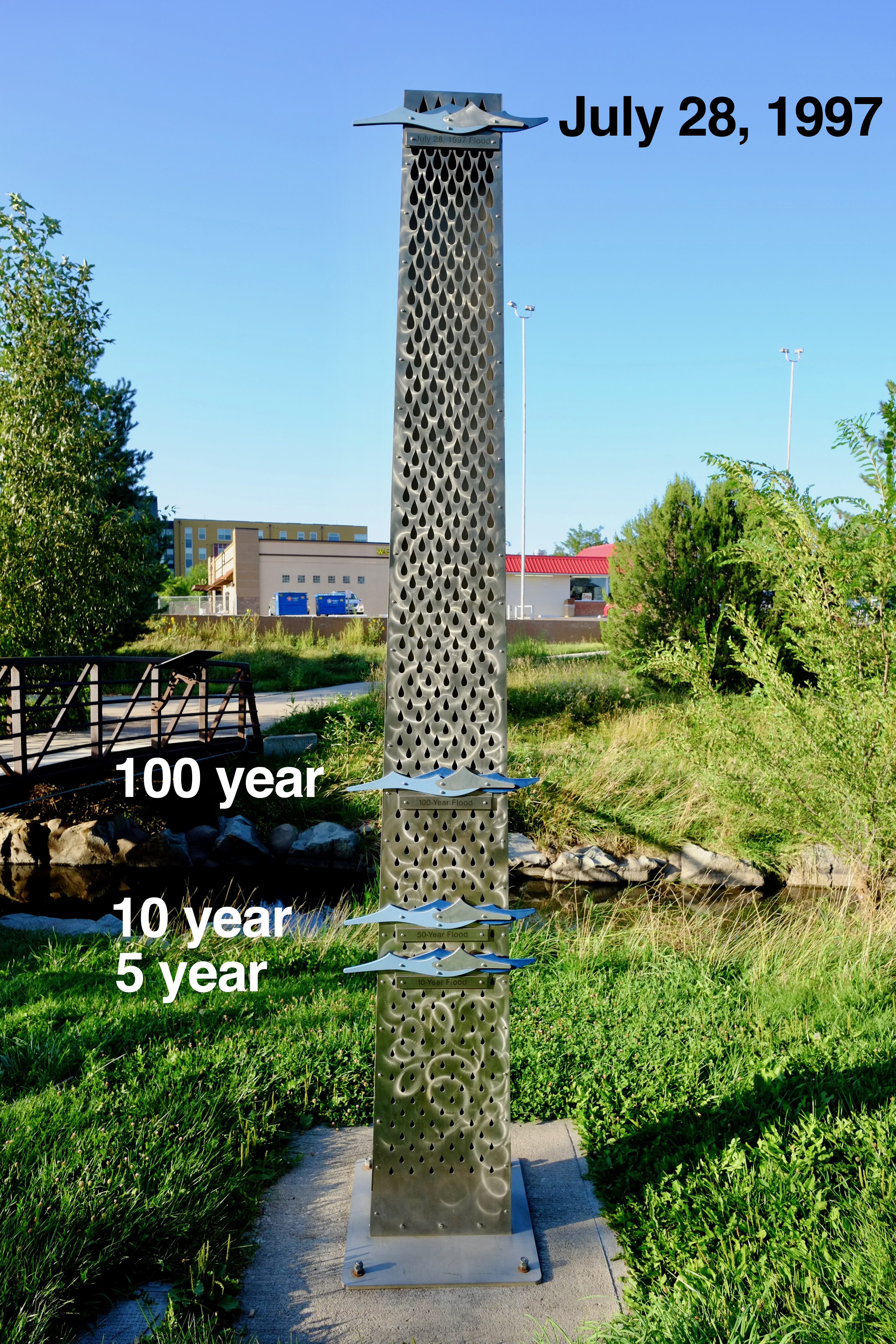{.lightbox #fig-marker width=50%}
For example, I often ride past a marker in
Creekside Park (@fig-marker) showing the magnitude of a severe flood on July 28, 1997
in Fort Collins. After a torrent of rain fell in a short period of time,
Spring Creek overflowed and washed out large areas of the community. Ultimately, the storm caused millions in property
damage, dozens of injuries, and five fatalities, and the experience led to many improvements in stormwater management and flood preparedness. The marker depicts the
unprecedented magnitude of the flood by comparing it to the much smaller
5-, 10-, and 100-year flood levels.
Despite its longstanding use in the physical sciences, the techniques
can also be used to understand biological phenomena. I first encountered
extreme value analysis in a
[study](https://doi.org/10.4319/lo.1990.35.1.0001) examining the
stochastic forces of crashing waves on limpets in rocky shores, and the
authors sought to quantify the probability of an extreme wave-induced
force potentially dislodging the aquatic snails. The cumulative density
function (CDF) for the Generalized Extreme Value (GEV) distribution can
be defined as:
$$F(x;\mu,\sigma,\gamma)=e^{-[1-\gamma(x-\mu)/\sigma]^{1/\gamma}}$$ {#eq-GEVD-CDF}
where $\gamma\ne0$ and $[1-\gamma(x-\mu)/\sigma]>0$. The three
parameters $\mu$, $\sigma$, and $\gamma$ depict the location, scale, and
shape of the distribution. The location parameter, $\mu$, represents the
most common, i.e., modal, extreme value. The scale parameter, $\sigma$,
portrays the rate of change in $x$ with the natural logarithm of time,
and the ration $\sigma/\gamma$ represents the maximum extreme value. The
return level, $x$, associated with a return period, $T$, corresponds to
the $1-p$ quantile of the distribution, where $p=1/T$. For example, a
100-year return level would correspond to the $1-{1\over100}=0.99$
quantile. Return levels can be obtained using the quantile function:
$$F^{-1}(1-p;\mu,\sigma,\gamma)=\mu+(\sigma/\gamma)\{{1\over[-ln(1-p)]^\gamma}-1\}$$ {#eq-quantile-function}
where $\gamma\ne0$. The interpretation of a return level often causes
confusion, but it is simply the value expected to be exceeded, on
average, once every $T$ years.
The `extRemes` package was developed by Eric Gilleland, a CSU graduate
now working at the National Center for Atmospheric Research in Boulder,
and it has facilitated greater interest and use of extreme value
statistics by many more people, including me! To update the data, I
consolidated the 20^th^ Century weather data from Fort Collins contained
in `extRemes` with more recent observations from the same weather
station. Today, the weather station is situated on the main campus of
CSU near the Lory Student Center, but the station was initially operated
near the former "Old Main" building with observations starting on 1
January 1889. Maintained by the Department of Atmospheric Science, the
station offers one of the oldest weather records in the state.
```{r libraries-data-graphics, echo=TRUE, warning=FALSE, error=FALSE}
#| code-fold: true
library(tidyverse)
library(ggtext)
library(extRemes)
library(gridExtra)
library(kableExtra)
library(httr)
library(jsonlite)
library(modelsummary)
library(showtext)

# Load FCwx data from extRemes package
data(FCwx)

# Query updated FCwx observations and combine
api <- GET("https://coagmet.colostate.edu/data/daily/fcl01.json?from=2000-01-01&to=2022-12-31&fields=tMax,tMin,precip")
FCwx2k <- do.call(cbind.data.frame,fromJSON(rawToChar(api$content))) |>
  mutate(dt = as.Date(time,"%Y-%m-%d"), Dy = yday(dt), Mn = month(dt), Year = year(dt)) |>
  select(dt,Dy,Mn,Year,tMin) |> rename(MnT = tMin)

FCwx <- FCwx |> mutate(dt = as.Date(paste(Dy,"-",Mn,"-",Year),"%d - %m - %Y")) |>
  select(dt,Dy,Mn,Year,MnT)

FCwx <- bind_rows(FCwx,FCwx2k) |> mutate(doy = yday(dt))
FCwx <- FCwx[FCwx$MnT != -999,]

#windowsFonts(Inter = windowsFont("Inter"))
font_add_google("Inter","inter")
showtext_auto()

theme_nice <- function() {
  theme_minimal(base_family = "inter") +
    theme(panel.grid.minor = element_blank(),
          panel.spacing.x = unit(25, "points"),
          plot.title = element_text(family= "inter", face = "bold"),
          axis.title = element_text(family = "inter"),
          strip.text = element_text(family = "inter", face = "bold",
                                    size = rel(1), hjust = 0),
          strip.background = element_rect(fill = "grey80", color = NA))
}

update_geom_defaults("label", list(family="inter"))
update_geom_defaults(ggtext::GeomRichText, list(family="inter"))
```
Upon inspection, the data revealed some obvious patterns. Between
`r min(format(FCwx$dt,"%Y"))` and `r max(format(FCwx$dt,"%Y"))`, there
were `r format(sum(FCwx$MnT < 32, na.rm = TRUE),big.mark=",")` days with
low temperatures below freezing in Fort Collins (approximately 44% of
all observed days). Recorded on
`r format(FCwx[FCwx$MnT == min(FCwx$MnT),1], "%d %B %Y")`, the coldest
daily low was `r min(FCwx$MnT)`° F! Wow, that's really cold. Near the
lower limit of the observed range, there were
`r sum(FCwx$MnT < -20, na.rm = TRUE)` days with low temperatures below
-20° F, but such extremely cold days were not observed uniformly over
the past 122 years:
`r round((nrow(FCwx |> filter(MnT < -20 & format(dt,"%Y") < 1950)) / sum(FCwx$MnT < -20, na.rm = TRUE)),3)*100`%
of the events occurred before 1950.
```{r global-plot, echo=TRUE, warning=FALSE, error=FALSE, fig.showtext= TRUE}
#| code-fold: true
#| label: fig-global-plot
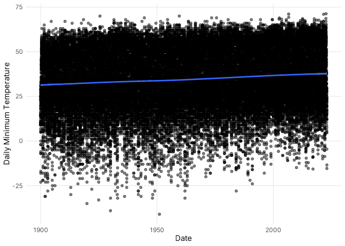
#| fig-cap: "Daily minimum temperatures in Fort Collins, CO between 1900 and 2022"
ggplot(data=FCwx,aes(x=dt,y=MnT)) +
  geom_point(alpha=0.5,position="jitter") +
  geom_smooth() +
  xlab("Date") + ylab("Daily Minimum Temperature") +
  theme_nice()
```
In the entire data record (@fig-global-plot), there is an obvious upward
trend in daily minimum temperatures over time, and you can also clearly
see more variability around the lower limit of observations. As a
convenient starting point, I simply fit a GEV distribution to all
observations. The location parameter for the preliminary fit, for
example, indicated that the most common daily minimum temperature was
41.6° F (@tbl-fit0). For such cases, one important modeling assumption
requires the use of homogeneous data obtained from a process *not*
undergoing any systematic change. In many cases, however, extreme value
processes exhibit slowly-varying or cyclical behavior, and the
probability of an extreme event, often, varies according to diurnal,
seasonal, or annual conditions. Apart from significant seasonal
variation, the long-term trend towards warmer daily low temperatures in
Fort Collins likely violates this assumption.
```{r initial-fit, echo=TRUE, warning=FALSE, error=FALSE}
#| code-fold: true
#| label: tbl-fit0
#| tbl-cap: "Parameter estimates for stationary Generalized Extreme Value distribution fit to negative daily minimum temperatures in Fort Collins, CO between 1900 and 2022"
# Fit stationary model
fit0 <- fevd(-MnT ~ 1, FCwx, type = "GEV", span = 123, units = "deg F", time.units = "days", period.basis = "year")
# Stationary model summary table
fit0.summary <- summary(fit0, silent=TRUE)
params.ci.fit0 <- data.frame(matrix(ci(fit0, type = "parameter"),ncol=3))
colnames(params.ci.fit0) <- c("ll","est","ul")
fit0.model.summary <- params.ci.fit0 |>
mutate(estimate = paste(round(params.ci.fit0$est,digits=2)," (",round(params.ci.fit0$ll,digits=2),", ",round(params.ci.fit0$ul,digits=2),")", sep = "")) |>
select(estimate)
fit0.model.summary <- data.frame(params = c("Location, μ","Scale, σ","Shape, γ"), fit0.model.summary)
footnote(kbl(fit0.model.summary, format="html", booktabs=TRUE, col.names=c("Parameters", "Estimate (95% CI)"), row.names=FALSE, digits=2, align="lc", escape=FALSE) |>
column_spec(1,width="10em") |>
column_spec(2,width="12em") |>
kable_styling(full_width = FALSE, position="left"), paste("Negative log-likelihood (NLLH): ",round(fit0$results$value,2),"; Bayesian Information Criterion (BIC): ",round(fit0.summary$BIC,2), sep=""), footnote_as_chunk = TRUE)
```
Fortunately, it is possible to account for non-stationary extremes by
directly modeling variation in the distribution parameters. To explore
variation in the distribution parameters over time, I fit multiple
stationary GEV distributions to short, overlapping five-year segments of
the data between 1902 and 2018.
```{r moving-fit, echo=TRUE, warning=FALSE, error=FALSE, fig.showtext=TRUE}
#| code-fold: true
#| label: fig-moving-fit
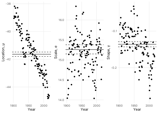
#| fig-cap: "Generalized Extreme Value distribution parameters fit to running five-year windows of daily minimum temperature in Fort Collins, CO between 1902 and 2018"
# Fit GEVD using running five-year windows between 1902 and 2018 and store result

mnt.yrs <- list()

for (i in 1902:2018){
  mnt.yrs[[i-1901]] <- fevd(-MnT ~ 1, FCwx |> filter(format(dt,"%Y") == seq(i-2,i+2)), type = "GEV", span = 5, units = "deg F", time.units = "days", period.basis = "year")
}

locs.yrs <- data.frame(years = seq(1902,2018),locations = matrix(unlist(lapply(mnt.yrs,'[[',c(20,1,1)))))
scls.yrs <- data.frame(years = seq(1902,2018),scales = matrix(unlist(lapply(mnt.yrs,'[[',c(20,1,2)))))
shps.yrs <- data.frame(years = seq(1902,2018),shapes = matrix(unlist(lapply(mnt.yrs,'[[',c(20,1,3)))))

p1 <- ggplot(data=locs.yrs, aes(x=years, y=locations)) +
  labs(x = "Year", y = "Location, \u03bc", escape = FALSE) +
  geom_hline(yintercept = -41.64) +
  geom_hline(yintercept = -41.8, linetype = "dashed") +
  geom_hline(yintercept = -41.48, linetype = "dashed") +
  geom_point() + theme_nice() +
  scale_x_continuous(breaks = c(1900, 1950, 2000))
p2 <- ggplot(data=scls.yrs, aes(x=years, y=scales)) +
  labs(x = "Year", y = "Scale, \u03c3") +
  geom_hline(yintercept = 15.26) +
  geom_hline(yintercept = 15.15, linetype = "dashed") +
  geom_hline(yintercept = 15.38, linetype = "dashed") +
  geom_point() + theme_nice() +
  scale_x_continuous(breaks = c(1900, 1950, 2000))
p3 <- ggplot(data=shps.yrs, aes(x=years, y=shapes)) +
  labs(x = "Year", y = "Shape, \u03b3") +
  geom_hline(yintercept = -0.136) +
  geom_hline(yintercept = -0.143, linetype = "dashed") +
  geom_hline(yintercept = -0.129, linetype = "dashed") +
  geom_point() + theme_nice() +
  scale_x_continuous(breaks = c(1900, 1950, 2000))
grid.arrange(p1,p2,p3,nrow=1)
```
The estimates show obvious variation in the location parameter over the
examined years with the modal (negative) daily low slowly decreasing
(increasing) over time. This is consistent with the trend towards warmer
daily minimum temperatures observed in @fig-global-plot. Compared to the
location parameter, the other two parameters do not similarly vary over
time. However, it's also completely obvious to expect seasonal variation
in daily minimum temperatures, and a simple harmonic function can be
used to model cyclical variation in seasonal lows. For the
non-stationary case, I fit two candidate models: one modelling annual
and seasonal variation in the location parameter and a second modelling
additional seasonal variation in the scale parameter. In both models,
the location parameter was modeled using:
$$\mu=\mu_0+\mu_1cos(2\pi*doy/365.25)+\mu_2sin(2\pi*doy/365.25)+\mu_3*year$$ {#eq-fit-1}
where $doy$ is the day of the year represented as an integer and $year$
is the calendar year.
```{r fit1-summary, echo=TRUE, warning=FALSE, error=FALSE}
#| code-fold: true
#| label: tbl-fit1
#| tbl-cap: "Parameter estimates for non-stationary Generalized Extreme Value distribution fit to negative daily minimum temperatures in Fort Collins, CO between 1900 and 2022"
# Non-stationary model 1
fit1 <- fevd(-MnT ~ 1, FCwx,location.fun = ~ cos(2*pi*doy/365.25) + sin(2*pi*doy/365.25) + Year, type = "GEV", span = 123, units = "deg F", time.units = "days", period.basis = "year")
# Non-stationary model 1 summary table
fit1.summary <- summary(fit1, silent=TRUE)
params.ci.fit1 <- data.frame(matrix(ci(fit1, type = "parameter"),ncol=3))
colnames(params.ci.fit1) <- c("ll","est","ul")
fit1.model.summary <- params.ci.fit1 |>
mutate(estimate = paste(round(params.ci.fit1$est,digits=2)," (",round(params.ci.fit1$ll,digits=2),", ",round(params.ci.fit1$ul,digits=2),")", sep = "")) |>
select(estimate)
fit1.model.summary <- data.frame(params = c("μ0", "μ1", "μ2", "μ3", "Scale, σ","Shape, γ"), fit1.model.summary)
footnote(kbl(fit1.model.summary, format="html", booktabs=TRUE, col.names=c("Parameters", "Estimate (95% CI)"), row.names=FALSE, digits=2, align="lc", escape=FALSE) |>
column_spec(1,width="10em") |>
column_spec(2,width="12em") |>
pack_rows("Location, μ", 1, 4, escape = FALSE) |>
kable_styling(full_width = FALSE, position = "left"), paste("Negative log-likelihood (NLLH): ",round(fit1$results$value,2),"; Bayesian Information Criterion (BIC): ",round(fit1.summary$BIC,2),"; See Equation 3 for the function used to model the location parameter.", sep = ""), footnote_as_chunk = TRUE)
```
Compared to the stationary model, the BIC is about 18% lower for the
non-stationary mode, indicating a much better fit when the annual and
seasonal variation in the location parameter was modeled. In the second
model, the scale parameter was additionally modeled using:
$$\sigma=\sigma_0+\sigma_1cos(2\pi*doy/365.25)+\sigma_2sin(2\pi*doy/365.25)$$ {#eq-fit-2}
```{r fit2-summary, echo=TRUE, warning=FALSE, error=FALSE}
#| code-fold: true
#| label: tbl-fit2
#| tbl-cap: "Parameter estimates for non-stationary Generalized Extreme Value distribution fit to negative daily minimum temperatures in Fort Collins, CO between 1900 and 2022"
# Non-stationary model 2
fit2 <- fevd(-MnT ~ 1, FCwx,location.fun = ~ cos(2*pi*doy/365.25) + sin(2*pi*doy/365.25) + Year, scale.fun = ~ cos(2*pi*doy/365.25) + sin(2*pi*doy/365.25), use.phi = TRUE, type = "GEV", span = 123, units = "deg F", time.units = "days", period.basis = "year")
# Non-stationary model 2 summary table
fit2.summary <- summary(fit2, silent=TRUE)
params.ci.fit2 <- data.frame(matrix(ci(fit2, type = "parameter"),ncol=3))
colnames(params.ci.fit2) <- c("ll","est","ul")
fit2.model.summary <- params.ci.fit2 |>
mutate(estimate = paste(round(params.ci.fit2$est,digits=2)," (",round(params.ci.fit2$ll,digits=2),", ",round(params.ci.fit2$ul,digits=2),")", sep = "")) |>
select(estimate)
fit2.model.summary <- data.frame(params = c("μ0", "μ1", "μ2", "μ3", "σ0", "σ1", "σ2", "Shape, γ"), fit2.model.summary)
footnote(kbl(fit2.model.summary, format="html", booktabs=TRUE, col.names=c("Parameters", "Estimate (95% CI)"), row.names=FALSE, digits=2, align="lc", escape=FALSE) |>
column_spec(1,width="10em") |>
column_spec(2,width="12em") |>
pack_rows("Location, μ", 1, 4, escape = FALSE) |>
pack_rows("Scale, σ", 5, 7, escape = FALSE) |>
kable_styling(full_width = FALSE, position = "left"), paste("Negative log-likelihood (NLLH): ",round(fit2$results$value,2),"; Bayesian Information Criterion (BIC): ",round(fit2.summary$BIC,2),"; See Equation 3 and Equation 4 for the functions used to model the location and scale parameter, respectively.", sep = ""), footnote_as_chunk = TRUE)
```
The fit statistics and model diagnostics generally suggest that the
second model is a better choice between the two non-stationary
candidates. The model could undoubtedly be improved to better fit the
data, but the current version depicts broad patterns in the data
reasonably well and allows for the exploration of model applications.
Using the non-stationary model, it is possible to estimate return
periods, return levels, and probabilities associated with extreme low
temperatures. For example, I could estimate the return period (or the
probability) for a -15° F freeze in late December. Instead, I estimated
the 100-year return levels for every day in March, April, October, and
November on five different years contained in the data: 1900, 1940,
1980, 2000, and 2020.
```{r return-levels, echo=TRUE, warning=FALSE, error=FALSE, fig.showtext=TRUE}
#| code-fold: true
#| label: fig-return-levels
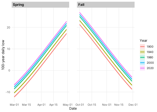
#| fig-cap: "Effective 100-year return levels for daily minimum temperatures in Fort Collins, CO on different dates"
v1 <- make.qcov(fit2, vals = list(mu1 = cos(2*pi*60:120/365.25), mu2 = sin(2*pi*60:120/365.25), mu3 = rep(1900,61), phi1 = cos(2*pi*60:120/365.25), phi2 = sin(2*pi*60:120/365.25)))
ci100YrRLevelsMarApr1900 <- data.frame(matrix(ci(fit2, type = "return.level", return.period = 100, qcov = v1),ncol=4))
colnames(ci100YrRLevelsMarApr1900) <- c("ll","est","ul","se")
v2 <- make.qcov(fit2, vals = list(mu1 = cos(2*pi*60:120/365.25), mu2 = sin(2*pi*60:120/365.25), mu3 = rep(1940,61), phi1 = cos(2*pi*60:120/365.25), phi2 = sin(2*pi*60:120/365.25)))
ci100YrRLevelsMarApr1940 <- data.frame(matrix(ci(fit2, type = "return.level", return.period = 100, qcov = v2),ncol=4))
colnames(ci100YrRLevelsMarApr1940) <- c("ll","est","ul","se")
v3 <- make.qcov(fit2, vals = list(mu1 = cos(2*pi*60:120/365.25), mu2 = sin(2*pi*60:120/365.25), mu3 = rep(1980,61), phi1 = cos(2*pi*60:120/365.25), phi2 = sin(2*pi*60:120/365.25)))
ci100YrRLevelsMarApr1980 <- data.frame(matrix(ci(fit2, type = "return.level", return.period = 100, qcov = v3),ncol=4))
colnames(ci100YrRLevelsMarApr1980) <- c("ll","est","ul","se")
v4 <- make.qcov(fit2, vals = list(mu1 = cos(2*pi*60:120/365.25), mu2 = sin(2*pi*60:120/365.25), mu3 = rep(2000,61), phi1 = cos(2*pi*60:120/365.25), phi2 = sin(2*pi*60:120/365.25)))
ci100YrRLevelsMarApr2000 <- data.frame(matrix(ci(fit2, type = "return.level", return.period = 100, qcov = v4),ncol=4))
colnames(ci100YrRLevelsMarApr2000) <- c("ll","est","ul","se")
v5 <- make.qcov(fit2, vals = list(mu1 = cos(2*pi*60:120/365.25), mu2 = sin(2*pi*60:120/365.25), mu3 = rep(2020,61), phi1 = cos(2*pi*60:120/365.25), phi2 = sin(2*pi*60:120/365.25)))
ci100YrRLevelsMarApr2020 <- data.frame(matrix(ci(fit2, type = "return.level", return.period = 100, qcov = v5),ncol=4))
colnames(ci100YrRLevelsMarApr2020) <- c("ll","est","ul","se")
v6 <- make.qcov(fit2, vals = list(mu1 = cos(2*pi*274:334/365.25), mu2 = sin(2*pi*274:334/365.25), mu3 = rep(1900,61), phi1 = cos(2*pi*274:334/365.25), phi2 = sin(2*pi*274:334/365.25)))
ci100YrRLevelsOctNov1900 <- data.frame(matrix(ci(fit2, type = "return.level", return.period = 100, qcov = v6),ncol=4))
colnames(ci100YrRLevelsOctNov1900) <- c("ll","est","ul","se")
v7 <- make.qcov(fit2, vals = list(mu1 = cos(2*pi*274:334/365.25), mu2 = sin(2*pi*274:334/365.25), mu3 = rep(1940,61), phi1 = cos(2*pi*274:334/365.25), phi2 = sin(2*pi*274:334/365.25)))
ci100YrRLevelsOctNov1940 <- data.frame(matrix(ci(fit2, type = "return.level", return.period = 100, qcov = v7),ncol=4))
colnames(ci100YrRLevelsOctNov1940) <- c("ll","est","ul","se")
v8 <- make.qcov(fit2, vals = list(mu1 = cos(2*pi*274:334/365.25), mu2 = sin(2*pi*274:334/365.25), mu3 = rep(1980,61), phi1 = cos(2*pi*274:334/365.25), phi2 = sin(2*pi*274:334/365.25)))
ci100YrRLevelsOctNov1980 <- data.frame(matrix(ci(fit2, type = "return.level", return.period = 100, qcov = v8),ncol=4))
colnames(ci100YrRLevelsOctNov1980) <- c("ll","est","ul","se")
v9 <- make.qcov(fit2, vals = list(mu1 = cos(2*pi*274:334/365.25), mu2 = sin(2*pi*274:334/365.25), mu3 = rep(2000,61), phi1 = cos(2*pi*274:334/365.25), phi2 = sin(2*pi*274:334/365.25)))
ci100YrRLevelsOctNov2000 <- data.frame(matrix(ci(fit2, type = "return.level", return.period = 100, qcov = v9),ncol=4))
colnames(ci100YrRLevelsOctNov2000) <- c("ll","est","ul","se")
v10 <- make.qcov(fit2, vals = list(mu1 = cos(2*pi*274:334/365.25), mu2 = sin(2*pi*274:334/365.25), mu3 = rep(2020,61), phi1 = cos(2*pi*274:334/365.25), phi2 = sin(2*pi*274:334/365.25)))
ci100YrRLevelsOctNov2020 <- data.frame(matrix(ci(fit2, type = "return.level", return.period = 100, qcov = v10),ncol=4))
colnames(ci100YrRLevelsOctNov2020) <- c("ll","est","ul","se")

ciRLevels <- rbind(ci100YrRLevelsMarApr1900,ci100YrRLevelsMarApr1940,ci100YrRLevelsMarApr1980,ci100YrRLevelsMarApr2000,ci100YrRLevelsMarApr2020,ci100YrRLevelsOctNov1900,ci100YrRLevelsOctNov1940,ci100YrRLevelsOctNov1980,ci100YrRLevelsOctNov2000,ci100YrRLevelsOctNov2020) |> mutate(Year = rep(factor(c(1900,1940,1980,2000,2020)),each=61,times=2), dt = rbind(data.frame(dt = rep(seq(as.Date("1900/03/01"),as.Date("1900/04/30"),by="days"),5)),data.frame(dt = rep(seq(as.Date("1900/10/01"),as.Date("1900/11/30"),by="days"),5))), Season = rep(factor(c("Spring","Fall")),each=305))

ciRLevels[,1:3] <- ciRLevels[,1:3] * -1

ggplot(data = ciRLevels, aes(x = dt$dt, y = est)) +
  geom_line(aes(color = Year), linewidth = 1) + geom_ribbon(aes(ymin=ll,ymax=ul,fill=Year),alpha=0.2) +
  xlab("Date") + ylab("100-year daily low") + facet_grid(~factor(Season, levels = c("Spring","Fall")), scales="free") +
  theme_nice()
```
The 100-year freezes estimated by the model follow a predictable warming
and cooling trend in the spring and fall (@fig-return-levels), respectively, but the return
levels also warmed considerably, by about 5° F, over each of the
evaluated decades. The confidence intervals are slightly larger during
dates closer to the winter months, reflecting the reduced variability in
daily lows during the warmer summer months.
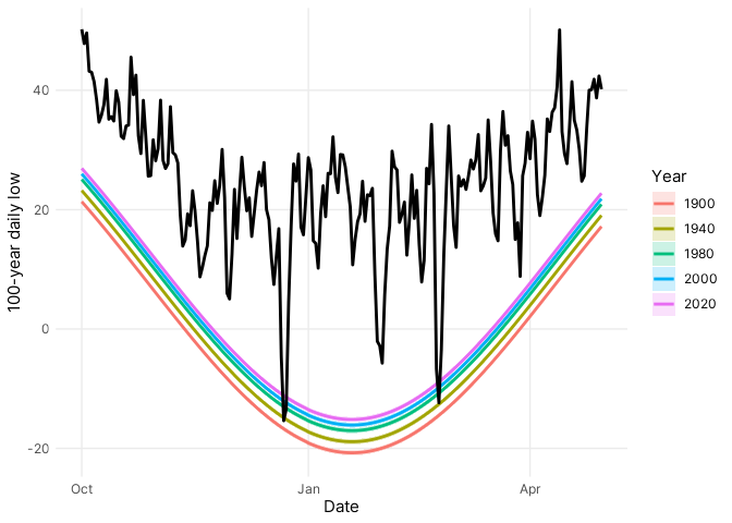
To evaluate the model predictions, I compared the 100-year return levels with daily minimum temperatures for the 2022-2023 winter season (@fig-validation), and the comparison clearly shows it was a cold winter with *two* 100-year freezes on 22 December and 23 February! On most days, however, the daily low temperatures were well above the severe freezes, consistent with expectations for extreme events.
```{r return-levels, echo=TRUE, warning=FALSE, error=FALSE, fig.showtext=TRUE}
#| code-fold: true
#| label: fig-validation
#| fig-cap: "Effective 100-year return levels for daily minimum temperatures (colored lines) in Fort Collins, CO compared to daily minimum temperatures during the 2022-2023 winter season (black line)"
v6 <- make.qcov(fit2, vals = list(mu1 = cos(2*pi*c(274:365,1:120)/365.25), mu2 = sin(2*pi*c(274:365,1:120)/365.25), mu3 = rep(1900,212), phi1 = cos(2*pi*c(274:365,1:120)/365.25), phi2 = sin(2*pi*c(274:365,1:120)/365.25)))
ci100YrRLevelsOctApr1900 <- data.frame(matrix(ci(fit2, type = "return.level", return.period = 100, qcov = v6),ncol=4))
colnames(ci100YrRLevelsOctApr1900) <- c("ll","est","ul","se")
v7 <- make.qcov(fit2, vals = list(mu1 = cos(2*pi*c(274:365,1:120)/365.25), mu2 = sin(2*pi*c(274:365,1:120)/365.25), mu3 = rep(1940,212), phi1 = cos(2*pi*c(274:365,1:120)/365.25), phi2 = sin(2*pi*c(274:365,1:120)/365.25)))
ci100YrRLevelsOctApr1940 <- data.frame(matrix(ci(fit2, type = "return.level", return.period = 100, qcov = v7),ncol=4))
colnames(ci100YrRLevelsOctApr1940) <- c("ll","est","ul","se")
v8 <- make.qcov(fit2, vals = list(mu1 = cos(2*pi*c(274:365,1:120)/365.25), mu2 = sin(2*pi*c(274:365,1:120)/365.25), mu3 = rep(1980,212), phi1 = cos(2*pi*c(274:365,1:120)/365.25), phi2 = sin(2*pi*c(274:365,1:120)/365.25)))
ci100YrRLevelsOctApr1980 <- data.frame(matrix(ci(fit2, type = "return.level", return.period = 100, qcov = v8),ncol=4))
colnames(ci100YrRLevelsOctApr1980) <- c("ll","est","ul","se")
v9 <- make.qcov(fit2, vals = list(mu1 = cos(2*pi*c(274:365,1:120)/365.25), mu2 = sin(2*pi*c(274:365,1:120)/365.25), mu3 = rep(2000,212), phi1 = cos(2*pi*c(274:365,1:120)/365.25), phi2 = sin(2*pi*c(274:365,1:120)/365.25)))
ci100YrRLevelsOctApr2000 <- data.frame(matrix(ci(fit2, type = "return.level", return.period = 100, qcov = v9),ncol=4))
colnames(ci100YrRLevelsOctApr2000) <- c("ll","est","ul","se")
v10 <- make.qcov(fit2, vals = list(mu1 = cos(2*pi*c(274:365,1:120)/365.25), mu2 = sin(2*pi*c(274:365,1:120)/365.25), mu3 = rep(2020,212), phi1 = cos(2*pi*c(274:365,1:120)/365.25), phi2 = sin(2*pi*c(274:365,1:120)/365.25)))
ci100YrRLevelsOctApr2020 <- data.frame(matrix(ci(fit2, type = "return.level", return.period = 100, qcov = v10),ncol=4))
colnames(ci100YrRLevelsOctApr2020) <- c("ll","est","ul","se")

ciRLevels <- rbind(ci100YrRLevelsOctApr1900,ci100YrRLevelsOctApr1940,ci100YrRLevelsOctApr1980,ci100YrRLevelsOctApr2000,ci100YrRLevelsOctApr2020) |> mutate(Year = rep(factor(c(1900,1940,1980,2000,2020)),each=212,times=1), dt = rbind(data.frame(dt = rep(seq(as.Date("2022/10/01"),as.Date("2023/04/30"),by="days"),5))))

ciRLevels[,1:3] <- ciRLevels[,1:3] * -1

api <- GET("https://coagmet.colostate.edu/data/daily/fcl01.json?from=2022-10-01&to=2023-04-30&fields=tMax,tMin,precip")
FCwx2223 <- do.call(cbind.data.frame,fromJSON(rawToChar(api$content))) |>
  mutate(dt = as.Date(time,"%Y-%m-%d"), Dy = yday(dt), Mn = month(dt), Year = year(dt)) |>
  select(dt,Dy,Mn,Year,tMin) |> rename(MnT = tMin)

ggplot(data = ciRLevels, aes(x = dt$dt, y = est)) +
  geom_line(aes(color = Year), linewidth = 1) + geom_ribbon(aes(ymin=ll,ymax=ul,fill=Year),alpha=0.2) +
  geom_line(data=FCwx2223,aes(x=dt, y=MnT), size=1) +
  xlab("Date") + ylab("100-year daily low") +
  theme_nice()
```